Testing Interactions in Nonlinear Regression

If the observations were independent (i.e., without blocks or repeated measurements), this model could be fitted using conventional nonlinear regression. My preference goes to drm() function in the ‘drc’ package (Ritz et al., 2015).

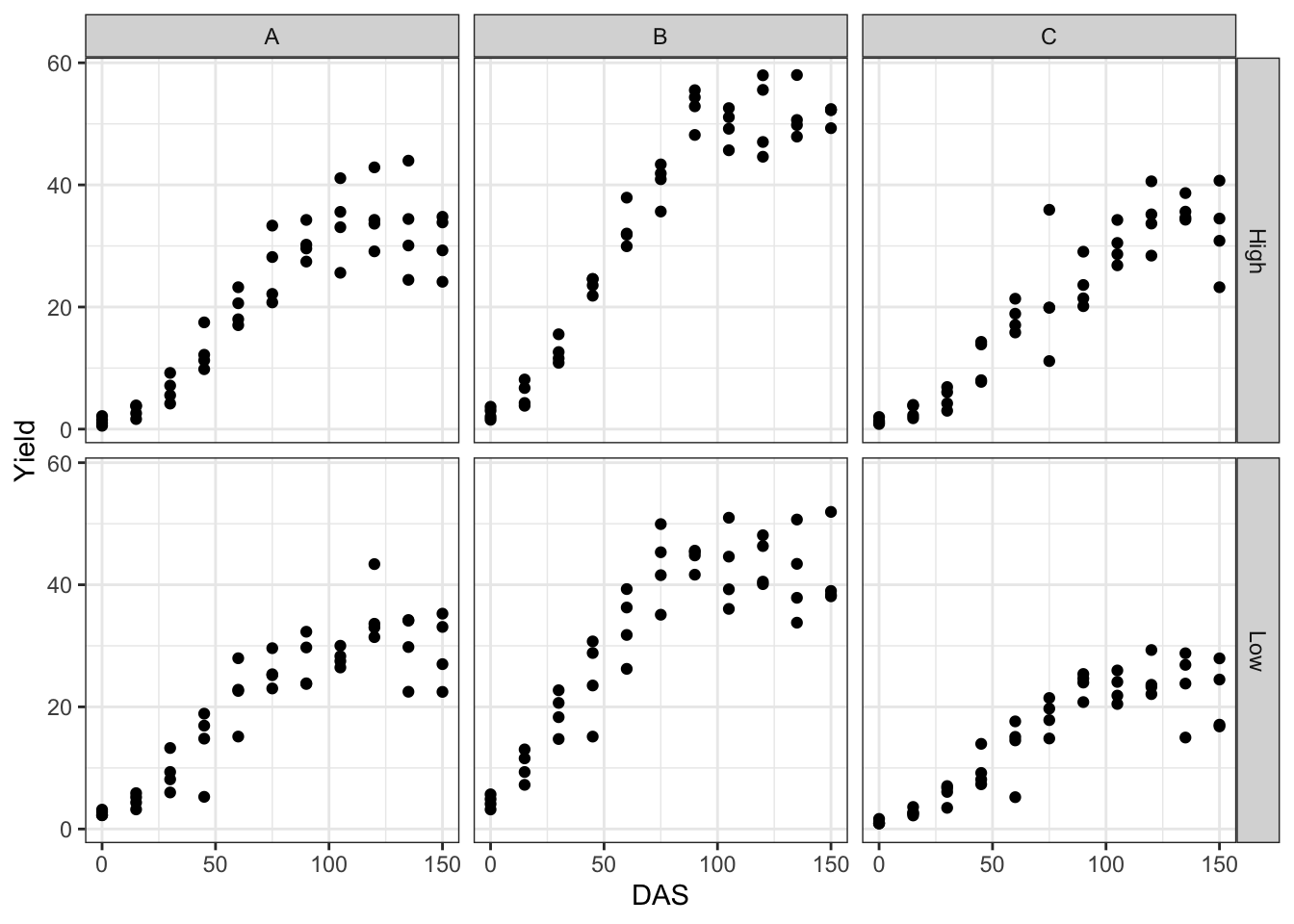
The coding is reported below: “Performance” is a function of (\(\sim\)) DAS, using a three-parameter logistic function (“fct = L.3()”). Different curves should be fitted for different combinations of genotypes and nitrogen levels (“curveid = N:GEN”), although these curves should be partly based on common parameter values (“pmodels = …).

The ‘pmodels’ argument requires some additional comments. It must be a vector with as many elements as there are parameters in the model (three, in this case: \(b\), \(d\) And \(e\)). Each element represents a linear function of variables and refers to the parameters in alphabetical order, i.e. the first element refers to \(b\)the second refers to \(d\) and the third to \(e\). The parameter \(b\) does not depend on any variable (“~ 1”) and therefore a constant value is adjusted to the curves; \(d\) And \(e\) depend on a fully factorial combination of genotype and nitrogen level (~N*GEN = ~N + GEN + N:GEN). Finally, we used the argument “bcVal = 0.5” to specify that we intend to use a two-sided transformation technique, in which a logarithmic transformation is performed for both sides of the equations. This is necessary to account for heteroskedasticity, but it does not affect the scale of the parameter estimates.

This model may be useful in other circumstances (no blocks and no repeated measurements), but it is wrong in our example. In fact, the observations are grouped within blocks and plots; by neglecting this, we violate the assumption of independence of the model residuals. Quick plots of the residuals against the fitted values and the QQ plot show that there are no problems with heteroscedasticity and normality, although a few outliers might merit careful inspection (which we will now neglect). Note that these two graphs are obtained using the plotRes() function in “statforbiology”.

Given the above, we need to use a different model here, although I will show that this naive adjustment can be useful.

Nonlinear mixed model fitting

To account for clustering of observations, we move to a nonlinear mixed effects (NLME) model. A good choice is nlme() function in the ‘nlme’ package (Pinheiro and Bates, 2000), although the syntax can sometimes be cumbersome. I will try to help, by listing and commenting on the most important arguments for this function. We need to specify the following:

A deterministic function. In this case we use the NLS.L3() function in the “statforbiology” package, which provides a logistic growth model with the same parameterization as the L.3() function in the ‘drc’ package.
Linear functions for model parameters. The ‘fixed’ argument in the ‘nlme’ function is very similar to the ‘pmodels’ argument in the ‘drm’ function above, in that it requires a list in which each element is a linear function of variables. The only difference is that the parameter name must be specified on the left side of the function.
Random effects for model parameters. These are specified using the “random” argument. In this case, the settings \(d\) And \(e\) should show random variability from block to block and from plot to plot, within a block. For the sake of simplicity, as a parameter \(b\) is not affected by genotype and nitrogen level, we also expect it to show no random variability between blocks and plots.
Starting values for model parameters. Autostart routines are not used by nlme() and so we need to specify a named vector, containing the initial values of the model parameters. In this case, I decided to use the result of the “naive” nonlinear regression above, which therefore turns out to be useful.

The transformation of both sides of the equation is done explicitly.

modnlme1 <- nlme(sqrt(Yield) ~ sqrt(NLS.L3(DAS, b, d, e)), 
                 data = dataset,
                    random = d + e ~ 1|Block/Plot,
                    fixed = list(b ~ 1, d ~ N*GEN, e ~ N*GEN),
                    start = coef(modNaive1), 
                 control = list(msMaxIter = 400))
summary(modnlme1)$tTable
##                     Value   Std.Error  DF    t-value      p-value
## b              0.05652837 0.002157629 228 26.1993018 1.044743e-70
## d.(Intercept) 33.91575348 1.222612866 228 27.7403865 5.073982e-75
## d.NLow        -3.18382830 1.592502935 228 -1.9992606 4.676721e-02
## d.GENB        18.90014651 1.864712716 228 10.1356881 3.602004e-20
## d.GENC        -1.15934033 1.686405282 228 -0.6874625 4.924901e-01
## d.NLow:GENB   -5.99216682 2.455759119 228 -2.4400467 1.544863e-02
## d.NLow:GENC   -5.82864845 2.217534809 228 -2.6284361 9.160826e-03
## e.(Intercept) 55.20071252 2.320784607 228 23.7853665 1.087153e-63
## e.NLow        -9.06217426 3.127165879 228 -2.8978873 4.123120e-03
## e.GENB        -4.47038042 2.761533544 228 -1.6188036 1.068720e-01
## e.GENC         4.00746125 3.084383627 228  1.2992746 1.951620e-01
## e.NLow:GENB   -4.71367457 4.055953633 228 -1.1621618 2.463848e-01
## e.NLow:GENC    2.23951067 4.609547644 228  0.4858417 6.275460e-01

From the graphs above we see that the overall fit is good. The fixed effects and variance components for the random effects are obtained as follows:

summary(modnlme1)$tTable
##                     Value   Std.Error  DF    t-value      p-value
## b              0.05652837 0.002157629 228 26.1993018 1.044743e-70
## d.(Intercept) 33.91575348 1.222612866 228 27.7403865 5.073982e-75
## d.NLow        -3.18382830 1.592502935 228 -1.9992606 4.676721e-02
## d.GENB        18.90014651 1.864712716 228 10.1356881 3.602004e-20
## d.GENC        -1.15934033 1.686405282 228 -0.6874625 4.924901e-01
## d.NLow:GENB   -5.99216682 2.455759119 228 -2.4400467 1.544863e-02
## d.NLow:GENC   -5.82864845 2.217534809 228 -2.6284361 9.160826e-03
## e.(Intercept) 55.20071252 2.320784607 228 23.7853665 1.087153e-63
## e.NLow        -9.06217426 3.127165879 228 -2.8978873 4.123120e-03
## e.GENB        -4.47038042 2.761533544 228 -1.6188036 1.068720e-01
## e.GENC         4.00746125 3.084383627 228  1.2992746 1.951620e-01
## e.NLow:GENB   -4.71367457 4.055953633 228 -1.1621618 2.463848e-01
## e.NLow:GENC    2.23951067 4.609547644 228  0.4858417 6.275460e-01
#
VarCorr(modnlme1)
##               Variance                     StdDev       Corr  
## Block =       pdLogChol(list(d ~ 1,e ~ 1))                    
## d.(Intercept) 3.933210e-08                 1.983232e-04 d.(In)
## e.(Intercept) 1.747130e-08                 1.321791e-04 -0.001
## Plot =        pdLogChol(list(d ~ 1,e ~ 1))                    
## d.(Intercept) 3.197539e-09                 5.654679e-05 d.(In)
## e.(Intercept) 9.573313e-10                 3.094077e-05 0     
## Residual      1.750623e-01                 4.184044e-01

Let us now return to our initial objective: to test the importance of the “genotype x nitrogen” interaction. Indeed, we have two tests: one for the parameter \(d\) and one for the parameter \(e\). First, we code two “reduced” models, where the effects of genotype and nitrogen are purely addictive. To do this, we change the fixed effects specification from ‘~N*GEN’ to ‘~N+GEN’. Also in this case, we use a “naive” nonlinear regression fit to obtain the starting values of the model parameters, to be used in the subsequent NLME model fit.

modNaive2 <- drm(Yield ~ DAS, fct = L.3(), 
                 data = dataset,
                 curveid = N:GEN,
                 pmodels = c( ~ 1,  ~ N + GEN,  ~ N * GEN), 
                 bcVal = 0.5)

modnlme2 <- nlme(sqrt(Yield) ~ sqrt(NLS.L3(DAS, b, d, e)), 
                 data = dataset,
                 random = d + e ~ 1|Block/Plot,
                 fixed = list(b ~ 1, d ~ N + GEN, e ~ N*GEN),
                 start = coef(modNaive2), 
                 control = list(msMaxIter = 200))

modNaive3 <- drm(Yield ~ DAS, fct = L.3(), data = dataset,
            curveid = N:GEN,
            pmodels = c( ~ 1,  ~ N*GEN,  ~ N + GEN), bcVal = 0.5)

modnlme3 <- nlme(sqrt(Yield) ~ sqrt(NLS.L3(DAS, b, d, e)),
                 data = dataset,
                 random = d + e ~ 1|Block/Plot,
                 fixed = list(b ~ 1, d ~ N*GEN, e ~ N + GEN),
                 start = coef(modNaive3), control = list(msMaxIter = 200))

Consider the first scale model ‘modnlme2’. In this model, the “genotype x nitrogen” interaction was removed for the \(d\) setting. We can compare this reduced model with the full model ‘modnlme1’, using a likelihood ratio test:

anova(modnlme1, modnlme2)
##          Model df      AIC      BIC    logLik   Test  L.Ratio p-value
## modnlme1     1 20 329.1496 400.6686 -144.5748                        
## modnlme2     2 18 334.2187 398.5857 -149.1093 1 vs 2 9.069075  0.0107

This test is significant, but the AIC value is very close for the two models. Considering that an LRT in mixed models is generally rather liberal, it should be possible to conclude that the “genotype x nitrogen” interaction is not significant and, therefore, the ranking of genotypes in terms of yield potential, as measured by the \(d\) The parameter must be independent of the nitrogen level.

Now consider the second model ‘modnlme3’. In this second model, the “genotype x nitrogen” interaction was removed for the “e” parameter. We can also compare this reduced model with the full model ‘modnlme1’, using a likelihood ratio test:

anova(modnlme1, modnlme3)
##          Model df      AIC      BIC    logLik   Test  L.Ratio p-value
## modnlme1     1 20 329.1496 400.6686 -144.5748                        
## modnlme3     2 18 328.2446 392.6117 -146.1223 1 vs 2 3.095068  0.2128

In this second test, the lack of significance of the “genotype x nitrogen” interaction seems less questionable than in the first.

I would like to conclude by drawing your attention to the ‘medrm’ function in the ‘medrc’ package, which can also be used to fit this type of nonlinear mixed effects models.

Happy coding with R! …and…don’t forget to check out my new book!

Professor Andrea Onofri
Department of Agricultural, Food and Environmental Sciences
University of Perugia (Italy)
Send your comments to: [email protected]

Book cover