Schotter plots in R | R-bloggers
Translating elements between languages reveals how each language approaches different design tradeoffs, and I think it’s a useful exercise. Having something to translate is the first step. I found a plot I wanted to generate, and some code that reproduced it, so here we go!
I don’t remember how I originally found this page (I didn’t keep a note on it, it seems) and it sat on my to-be-posted pile for too long, so here is the post I intended to write.
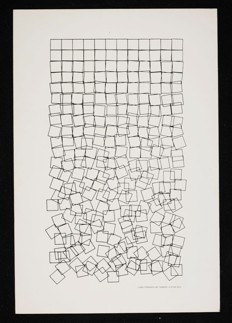
This article details the ALGOL code that generates Georg Nees’ 1968 computer-generated art “Schotter”, which shows a grid of squares that are increasingly moved in position and rotation.
1   'BEGIN''COMMENT'SCHOTTER.,
2   'REAL'R,PIHALB,PI4T.,
3   'INTEGER'I.,
4   'PROCEDURE'QUAD.,
5   'BEGIN'
6   'REAL'P1,Q1,PSI.,'INTEGER'S.,

7   JE1.=5*1/264.,JA1.=-JE1.,
8   JE2.=PI4T*(1+I/264).,JA2.=PI4T*(1-I/264).,
9   P1.=P+5+J1.,Q1.=Q+5+J1.,PS1.=J2.,
10  LEER(P1+R*COS(PSI),Q1+R*SIN(PSI)).,
11  'FOR'S.=1'STEP'1'UNTIL'4'DO'
12  'BEGIN'PSI.=PSI+PIHALB.,
13  LINE(P1+R*COS(PSI),Q1+R*SIN(PSI)).,
14  'END".,I.=I+1
15  'END'QUAD.,
16  R.=5*1.4142.,
17  PIHALB.=3.14159*.5.,P14T.=PIHALB*.5.,
18  I.=0.,
19  SERIE(10.0,10.0,22,12,QUAD)
20  'END' SCHOTTER.,

1   'REAL'P,Q,P1,Q1,XM,YM,HOR,VER,JLI,JRE,JUN,JOB.,
5   'INTEGER'I,M,M,T.,
7   'PROCEDURE'SERIE(QUER,HOCH,XMAL,YMAL,FIGUR).,
8   'VALUE'QUER,HOCH,XMAL,YMAL.,
9   'REAL'QUER,HOCH.,
10  'INTEGER'XMAL,YMAL.,
11  'PROCEDURE'FIGUR.,
12  'BEGIN'
13  'REAL'YANF.,
14  'INTEGER'COUNTX,COUNTY.,
15  P.=-QUER*XMAL*.5.,
16  Q.=YANF.=-HOCH*YMAL*.5.,
17  'FOR'COUNTX.=1'STEP'1'UNTIL'XMAL'DO'
18  'BEGIN'Q.=YANF.,
19  'FOR'COUNTY.=1'STEP'1'UNTIL'YMAL'DO'
20  'BEGIN'FIGUR.,Q.=Q+HOCH
21  'END'.,P.=P+QUER
22  'END'.,
23  LEER(-148.0,-105.0).,CLOSE.,
24  SONK(11).,
25  OPBEN(X,Y)
26  'END'SERIE.,

gravel
What is missing in this ALGOL code are the seeds necessary for the reproduction of the plot. The author went down a rabbit hole to investigate and calculate different values, but managed to determine them to be “(1922110153) for the x and y shift seed, and (1769133315) for the rotation seed”. They also provided a Python translation
import math
import drawsvg as draw

class Random:
    def __init__(self, seed):
        self.JI = seed

    def next(self, JA, JE):
        self.JI = (self.JI * 5) % 2147483648
        return self.JI / 2147483648 * (JE-JA) + JA

def draw_square(g, x, y, i, r1, r2):
    r = 5 * 1.4142
    pi = 3.14159
    move_limit = 5 * i / 264
    twist_limit = pi/4 * i / 264

    y_center = y + 5 + r1.next(-move_limit, move_limit)
    x_center = x + 5 + r1.next(-move_limit, move_limit)
    angle = r2.next(pi/4 - twist_limit, pi/4 + twist_limit)

    p = draw.Path()
    p.M(x_center + r * math.sin(angle), y_center + r * math.cos(angle))
    for step in range(4):
        angle += pi / 2
        p.L(x_center + r * math.sin(angle), y_center + r * math.cos(angle))
    g.append(p)

def draw_plot(x_size, y_size, x_count, y_count, s1, s2):
    r1 = Random(s1)
    r2 = Random(s2)
    d = draw.Drawing(180, 280, origin='center', style="background-color:#eae6e2")
    g = draw.Group(stroke='#41403a', stroke_width='0.4', fill='none',
                   stroke_linecap="round", stroke_linejoin="round")

    y = -y_size * y_count * 0.5
    x0 = -x_size * x_count * 0.5
    i = 0

    for _ in range(y_count):
        x = x0
        for _ in range(x_count):
            draw_square(g, x, y, i, r1, r2)
            x += x_size
            i += 1
        y += y_size
    d.append(g)
    return d

d = draw_plot(10.0, 10.0, 12, 22, 1922110153, 1769133315).set_render_size(w=500)
print(d.as_svg())
I wanted to see if I could also translate this into R – base plot I can draw line segments very well, and I was curious to color the squares in my own way.
Most of this code translates simply, except that the “randomness” is actually a sequence of values, starting with a specific seed. I recently talked about an old article of mine that (abusively) uses the set.seed() function to generate specific “random” words
printStr <- function(str) paste(str, collapse="")

set.seed(2505587); x <- sample(LETTERS, 5, replace=TRUE)
set.seed(11135560);y <- sample(LETTERS, 5, replace=TRUE)

paste(printStr(x), printStr(y))
## [1] "HELLO WORLD"
which I wanted to revisit based on an article by Andrew Heiss.
THE Random The class in this Python translation produces an iterator that returns a “next” value each time it is called with a specific “seed” and two values
class Random:
    def __init__(self, seed):
        self.JI = seed

    def next(self, JA, JE):
        self.JI = (self.JI * 5) % 2147483648
        return self.JI / 2147483648 * (JE-JA) + JA

r = Random(1)
r.next(2, 3)
## 2.0000000023283064
r.next(2, 3)
## 2.000000011641532
r.next(2, 3)
## 2.000000058207661
with the added complexity that subsequent calls update the seed itself.
When I first saw this, my mind went back to reading the “original” R paper “R: A Language for Data Analysis and Graphics” by Ross Ihaka and Robert Gentleman, in which I remember seeing the cool example of an OO system maintaining (non-global) state via <<-


Maintain the status of the total balance internal to the function
With this same trick, we can write an equivalent of Random class that also updates the seed internally
random <- function(seed)
  list(
    nextval = function(a, b)
      seed <<- (seed * 5) %% 2147483648
      seed / 2147483648 * (b-a) + a

  )


r <- random(1)
print(r$nextval(2, 3), digits = 16)
## [1] 2.000000002328306
print(r$nextval(2, 3), digits = 16)
## [1] 2.000000011641532
print(r$nextval(2, 3), digits = 16)
## [1] 2.000000058207661
Cool!
The rest of the translation mostly aligns with the base plot syntax.
This is what I ended up with
draw_square <- function(x, y, i, r1, r2, col)
  r = 5 * 1.4142
  move_limit = 5 * i / 264
  twist_limit = pi/4 * i / 264

  y_center = y + 5 + r1$nextval(-move_limit, move_limit)
  x_center = x + 5 + r1$nextval(-move_limit, move_limit)
  angle = r2$nextval(pi/4 - twist_limit, pi/4 + twist_limit)

  x0 <- x_center + r * sin(angle)
  y0 <- y_center + r * cos(angle)

  for (step in 1:4)
    angle <- angle + pi / 2
    x1 <- x_center + r * sin(angle)
    y1 <- y_center + r * cos(angle)
    segments(x0, y0, x1, y1, lwd = 1.75, col = col)
    x0 <- x1
    y0 <- y1


draw_plot <- function(x_size, y_size, x_count, y_count, s1, s2)
  r1 = random(s1)
  r2 = random(s2)

  plot(NULL, NULL, xlim = c(-60, 60), ylim = c(120, -120), axes = FALSE, ann = FALSE)

  y = -y_size * y_count * 0.5
  x0 = -x_size * x_count * 0.5
  i = 0

  for (z in 1:y_count)
    x = x0
    for (zz in 1:x_count)
      draw_square(x, y, i, r1, r2, "black")
      x <- x + x_size
      i <- i + 1

    y <- y + y_size


draw_plot(10.0, 10.0, 12, 22, 1922110153, 1769133315)

Figure 1: “Gravel” in R
Which uses the special seeds discovered in this original post. Checking the rotations, this does indeed appear to match the original art.
But why stop there? Now that I can trace it, I can change things…what if I used a different set of seeds, for example swapping them?
draw_plot(10.0, 10.0, 12, 22, 1769133315, 1922110153)

Figure 2: ‘Schotter’ in R with swapped seeds
or completely different values?
draw_plot(10.0, 10.0, 12, 22, 12345, 67890)

Figure 3: ‘Schotter’ in R with new seeds
What if we changed the colors? I could plot the color based on the progress on the grid, which seems pretty cool to me.
draw_plot <- function(x_size, y_size, x_count, y_count, s1, s2)
  r1 = random(s1)
  r2 = random(s2)

  plot(NULL, NULL, xlim = c(-60, 60), ylim = c(120, -120), axes = FALSE, ann = FALSE)

  y = -y_size * y_count * 0.5
  x0 = -x_size * x_count * 0.5
  i = 0

  for (z in 1:y_count)
    x = x0
    rcol <- scales::viridis_pal(option = "viridis")(y_count)[z]
    for (zz in 1:x_count)
      draw_square(x, y, i, r1, r2, rcol)
      x <- x + x_size
      i <- i + 1

    y <- y + y_size


draw_plot(10.0, 10.0, 12, 22, 1922110153, 1769133315)

Figure 4: ‘Schotter’ in R with viridis colors
Since writing this article, I have seen other examples of similar work. This tool demonstrated a simplified version
suppressPackageStartupMessages(library(tidyverse))
crossing(x=0:10, y=x) |>
  mutate(dx = rnorm(n(), 0, (y/20)^1.5),
         dy = rnorm(n(), 0, (y/20)^1.5)) |>
  ggplot() +
  geom_tile(aes(x=x+dx, y=y+dy, fill=y), colour='black',
            lwd=2, width=1, height=1, alpha=0.8, show.legend=FALSE) +
  scale_fill_gradient(high='#9f025e', low='#f9c929') +
  scale_y_reverse() + theme_void()
while this one showed a book ‘Crisis Engineering’ with a similar idea

Cover of “Crisis Engineering”
I’m sure I’ve seen others too.
It was a fun exploration of artistically inspired code translation, and I got to stretch my “maintaining internal state” muscles a bit. I have no doubt that someone more artistic than me could do much more.
As always, I can be found on Mastodon and in the comments section below.
devtools::session_info()
## ─ Session info ───────────────────────────────────────────────────────────────
##  setting  value
##  version  R version 4.5.3 (2026-03-11)
##  os       macOS Tahoe 26.3.1
##  system   aarch64, darwin20
##  ui       X11
##  language (EN)
##  collate  en_US.UTF-8
##  ctype    en_US.UTF-8
##  tz       Australia/Adelaide
##  date     2026-04-17
##  pandoc   3.6.3 @ /Applications/RStudio.app/Contents/Resources/app/quarto/bin/tools/aarch64/ (via rmarkdown)
##  quarto   1.7.31 @ /usr/local/bin/quarto
##
## ─ Packages ───────────────────────────────────────────────────────────────────
##  package      * version date (UTC) lib source
##  blogdown       1.23    2026-01-18 [1] CRAN (R 4.5.2)
##  bookdown       0.46    2025-12-05 [1] CRAN (R 4.5.2)
##  bslib          0.10.0  2026-01-26 [1] CRAN (R 4.5.2)
##  cachem         1.1.0   2024-05-16 [1] CRAN (R 4.5.0)
##  cli            3.6.5   2025-04-23 [1] CRAN (R 4.5.0)
##  devtools       2.4.6   2025-10-03 [1] CRAN (R 4.5.0)
##  digest         0.6.39  2025-11-19 [1] CRAN (R 4.5.2)
##  dplyr        * 1.2.0   2026-02-03 [1] CRAN (R 4.5.2)
##  ellipsis       0.3.2   2021-04-29 [1] CRAN (R 4.5.0)
##  evaluate       1.0.5   2025-08-27 [1] CRAN (R 4.5.0)
##  farver         2.1.2   2024-05-13 [1] CRAN (R 4.5.0)
##  fastmap        1.2.0   2024-05-15 [1] CRAN (R 4.5.0)
##  forcats      * 1.0.1   2025-09-25 [1] CRAN (R 4.5.0)
##  fs             1.6.7   2026-03-06 [1] CRAN (R 4.5.2)
##  generics       0.1.4   2025-05-09 [1] CRAN (R 4.5.0)
##  ggplot2      * 4.0.2   2026-02-03 [1] CRAN (R 4.5.2)
##  glue           1.8.0   2024-09-30 [1] CRAN (R 4.5.0)
##  gtable         0.3.6   2024-10-25 [1] CRAN (R 4.5.0)
##  hms            1.1.4   2025-10-17 [1] CRAN (R 4.5.0)
##  htmltools      0.5.9   2025-12-04 [1] CRAN (R 4.5.2)
##  jquerylib      0.1.4   2021-04-26 [1] CRAN (R 4.5.0)
##  jsonlite       2.0.0   2025-03-27 [1] CRAN (R 4.5.0)
##  knitr          1.51    2025-12-20 [1] CRAN (R 4.5.2)
##  labeling       0.4.3   2023-08-29 [1] CRAN (R 4.5.0)
##  lattice        0.22-9  2026-02-09 [1] CRAN (R 4.5.3)
##  lifecycle      1.0.5   2026-01-08 [1] CRAN (R 4.5.2)
##  lubridate    * 1.9.5   2026-02-04 [1] CRAN (R 4.5.2)
##  magrittr       2.0.4   2025-09-12 [1] CRAN (R 4.5.0)
##  Matrix         1.7-4   2025-08-28 [1] CRAN (R 4.5.3)
##  memoise        2.0.1   2021-11-26 [1] CRAN (R 4.5.0)
##  otel           0.2.0   2025-08-29 [1] CRAN (R 4.5.0)
##  pillar         1.11.1  2025-09-17 [1] CRAN (R 4.5.0)
##  pkgbuild       1.4.8   2025-05-26 [1] CRAN (R 4.5.0)
##  pkgconfig      2.0.3   2019-09-22 [1] CRAN (R 4.5.0)
##  pkgload        1.5.0   2026-02-03 [1] CRAN (R 4.5.2)
##  png            0.1-9   2026-03-15 [1] CRAN (R 4.5.2)
##  purrr        * 1.2.1   2026-01-09 [1] CRAN (R 4.5.2)
##  R6             2.6.1   2025-02-15 [1] CRAN (R 4.5.0)
##  RColorBrewer   1.1-3   2022-04-03 [1] CRAN (R 4.5.0)
##  Rcpp           1.1.1   2026-01-10 [1] CRAN (R 4.5.2)
##  readr        * 2.2.0   2026-02-19 [1] CRAN (R 4.5.2)
##  remotes        2.5.0   2024-03-17 [1] CRAN (R 4.5.0)
##  reticulate     1.45.0  2026-02-13 [1] CRAN (R 4.5.2)
##  rlang          1.1.7   2026-01-09 [1] CRAN (R 4.5.2)
##  rmarkdown      2.30    2025-09-28 [1] CRAN (R 4.5.0)
##  rstudioapi     0.18.0  2026-01-16 [1] CRAN (R 4.5.2)
##  S7             0.2.1   2025-11-14 [1] CRAN (R 4.5.2)
##  sass           0.4.10  2025-04-11 [1] CRAN (R 4.5.0)
##  scales         1.4.0   2025-04-24 [1] CRAN (R 4.5.0)
##  sessioninfo    1.2.3   2025-02-05 [1] CRAN (R 4.5.0)
##  stringi        1.8.7   2025-03-27 [1] CRAN (R 4.5.0)
##  stringr      * 1.6.0   2025-11-04 [1] CRAN (R 4.5.0)
##  tibble       * 3.3.1   2026-01-11 [1] CRAN (R 4.5.2)
##  tidyr        * 1.3.2   2025-12-19 [1] CRAN (R 4.5.2)
##  tidyselect     1.2.1   2024-03-11 [1] CRAN (R 4.5.0)
##  tidyverse    * 2.0.0   2023-02-22 [1] CRAN (R 4.5.0)
##  timechange     0.4.0   2026-01-29 [1] CRAN (R 4.5.2)
##  tzdb           0.5.0   2025-03-15 [1] CRAN (R 4.5.0)
##  usethis        3.2.1   2025-09-06 [1] CRAN (R 4.5.0)
##  vctrs          0.7.1   2026-01-23 [1] CRAN (R 4.5.2)
##  viridisLite    0.4.3   2026-02-04 [1] CRAN (R 4.5.2)
##  withr          3.0.2   2024-10-28 [1] CRAN (R 4.5.0)
##  xfun           0.56    2026-01-18 [1] CRAN (R 4.5.2)
##  yaml           2.3.12  2025-12-10 [1] CRAN (R 4.5.2)
##
##  [1] /Library/Frameworks/R.framework/Versions/4.5-arm64/Resources/library
##  * ── Packages attached to the search path.
##
## ─ Python configuration ───────────────────────────────────────────────────────
##  python:         /Users/jono/.cache/uv/archive-v0/3n3euDImmjsw3EYTJjfeY/bin/python
##  libpython:      /Users/jono/.local/share/uv/python/cpython-3.12.12-macos-aarch64-none/lib/libpython3.12.dylib
##  pythonhome:     /Users/jono/.cache/uv/archive-v0/3n3euDImmjsw3EYTJjfeY:/Users/jono/.cache/uv/archive-v0/3n3euDImmjsw3EYTJjfeY
##  virtualenv:     /Users/jono/.cache/uv/archive-v0/3n3euDImmjsw3EYTJjfeY/bin/activate_this.py
##  version:        3.12.12 (main, Oct 28 2025, 11:52:25) [Clang 20.1.4 ]
##  numpy:          /Users/jono/.cache/uv/archive-v0/3n3euDImmjsw3EYTJjfeY/lib/python3.12/site-packages/numpy
##  numpy_version:  2.4.4
##
##  NOTE: Python version was forced by VIRTUAL_ENV
##
## ──────────────────────────────────────────────────────────────────────────────
Related
PakarPBN
A Private Blog Network (PBN) is a collection of websites that are controlled by a single individual or organization and used primarily to build backlinks to a “money site” in order to influence its ranking in search engines such as Google. The core idea behind a PBN is based on the importance of backlinks in Google’s ranking algorithm. Since Google views backlinks as signals of authority and trust, some website owners attempt to artificially create these signals through a controlled network of sites.
In a typical PBN setup, the owner acquires expired or aged domains that already have existing authority, backlinks, and history. These domains are rebuilt with new content and hosted separately, often using different IP addresses, hosting providers, themes, and ownership details to make them appear unrelated. Within the content published on these sites, links are strategically placed that point to the main website the owner wants to rank higher. By doing this, the owner attempts to pass link equity (also known as “link juice”) from the PBN sites to the target website.
The purpose of a PBN is to give the impression that the target website is naturally earning links from multiple independent sources. If done effectively, this can temporarily improve keyword rankings, increase organic visibility, and drive more traffic from search results.
Related Posts

The DX shift no one noticed: Web interoperability

7 Basement Floor Plans for Contractors & Builders Managing Modern Basement Construction Projects – Blog
