Conformalized TabPFN: prediction intervals for a pre-trained transformer for tabular data in Python and R

Knowing a model’s prediction is useful. Knowing how reliable this prediction is, it is even more so. Conformal prediction provides just that: statistically valid prediction intervals with guaranteed coverage (under certain conditions), regardless of the underlying model or data distribution.

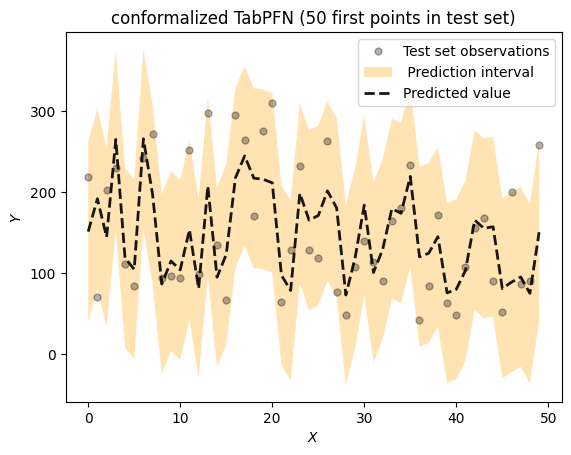
In this article, we combine two powerful tools: TabPFNA pretrained transformer for tabular dataAnd nnetsauce‘s PredictionInterval (which implements Split Conformal Prediction), which wraps any scikit-learn compatible regressor into a conformal predictor. We demonstrate the full pipeline on the diabetes dataset, first in Python and then in R via reticulate. Both versions produce identical results: a coverage rate of 96.7% at the nominal level of 95%.

!pip install tabpfn tabpfn_client

!pip install nnetsauce

import tabpfn_client

API_TOKEN = "" # <- Paste your TabPFN token here (from 


tabpfn_client.set_access_token(API_TOKEN)

from sklearn.datasets import load_diabetes
from sklearn.model_selection import train_test_split
from tabpfn_client import TabPFNRegressor
from sklearn.metrics import mean_squared_error
import numpy as np

reg = TabPFNRegressor()

X, y = load_diabetes(return_X_y=True)
X_train, X_test, y_train, y_test = train_test_split(X, y, test_size=0.2, random_state=42)

reg.fit(X_train, y_train)
preds = reg.predict(X_test)
rmse = np.sqrt(mean_squared_error(y_test, preds))
print(-rmse)

00:00 Fitting... |

WARNING:tabpfn_client.client:The provided train set hashes match previously uploaded train sets.


00:00 Fitting... Done!
00:00 Predicting... -

WARNING:tabpfn_client.client:The provided test set hash matches a previously uploaded test set.


00:01 Predicting... Done!
-51.559912022529886

import nnetsauce as ns

reg_conformal = ns.PredictionInterval(reg, level=95)
reg_conformal.fit(X_train, y_train)
preds = reg_conformal.predict(X_test, return_pi=True)

00:00 Fitting... |

WARNING:tabpfn_client.client:The provided train set hashes match previously uploaded train sets.


00:00 Fitting... Done!
00:00 Predicting... -

WARNING:tabpfn_client.client:The provided test set hash matches a previously uploaded test set.


00:01 Predicting... Done!
00:00 Predicting... -

WARNING:tabpfn_client.client:The provided test set hash matches a previously uploaded test set.


00:01 Predicting... Done!
00:00 Predicting... -

WARNING:tabpfn_client.client:The provided test set hash matches a previously uploaded test set.


00:01 Predicting... Done!

print(f"coverage_rate: np.mean((preds.lower<=y_test)*(preds.upper>=y_test))")

coverage_rate: 0.9662921348314607

import warnings
import matplotlib.pyplot as plt


warnings.filterwarnings('ignore')

split_color="green"
split_color2 = 'orange'
local_color="gray"

def plot_func(x,
              y,
              y_u=None,
              y_l=None,
              pred=None,
              shade_color="",
              method_name="",
              title=""):

    fig = plt.figure()

    plt.plot(x, y, 'k.', alpha=.3, markersize=10,
             fillstyle="full", label=u'Test set observations')

    if (y_u is not None) and (y_l is not None):
        plt.fill(np.concatenate([x, x[::-1]]),
                 np.concatenate([y_u, y_l[::-1]]),
                 alpha=.3, fc=shade_color, ec="None",
                 label = method_name + ' Prediction interval')

    if pred is not None:
        plt.plot(x, pred, 'k--', lw=2, alpha=0.9,
                 label=u'Predicted value')

    #plt.ylim([-2.5, 7])
    plt.xlabel('$X$')
    plt.ylabel('$Y$')
    plt.legend(loc="upper right")
    plt.title(title)

    plt.show()


max_idx = 50
plot_func(x = range(max_idx),
          y = y_test[0:max_idx],
          y_u = preds.upper[0:max_idx],
          y_l = preds.lower[0:max_idx],
          pred = preds.mean[0:max_idx],
          shade_color=split_color2,
          title = f"conformalized TabPFN (max_idx first points in test set)")

For this R version, I used R in the same notebook as Python, in Google Colab.

%load_ext rpy2.ipython

%R install.packages("reticulate")

%%R

# Conformalized TabPFN in R via reticulate

library(reticulate)

# ── 0. Python environment ──────────────────────────────────────────────────────
# Use your preferred Python env. Uncomment one (automatic on Google Colab):
# use_python("/usr/bin/python3")
# use_virtualenv("r-tabpfn")
# use_condaenv("r-tabpfn")

# Install required packages into the active Python env (run once)
# py_install(c("tabpfn", "tabpfn_client", "nnetsauce", "scikit-learn",
#              "matplotlib", "numpy"), pip = TRUE)

# ── 1. Imports ─────────────────────────────────────────────────────────────────
sklearn_datasets  <- import("sklearn.datasets")
sklearn_model_sel <- import("sklearn.model_selection")
sklearn_metrics   <- import("sklearn.metrics")
tabpfn_client     <- import("tabpfn_client")
ns                <- import("nnetsauce")
np                <- import("numpy")
plt               <- import("matplotlib.pyplot")
warnings          <- import("warnings")

# ── 2. TabPFN API token ────────────────────────────────────────────────────────
API_TOKEN <- ""   # <-- paste your TabPFN token here (from 
tabpfn_client$set_access_token(API_TOKEN)

TabPFNRegressor <- tabpfn_client$TabPFNRegressor

# ── 3. Data ────────────────────────────────────────────────────────────────────
diabetes   <- sklearn_datasets$load_diabetes(return_X_y = TRUE)
X          <- diabetes[[1]]
y          <- diabetes[[2]]

split      <- sklearn_model_sel$train_test_split(X, y, test_size = 0.2, random_state = 42L)
X_train    <- split[[1]]
X_test     <- split[[2]]
y_train    <- split[[3]]
y_test     <- split[[4]]

# ── 4. Fit TabPFN regressor ────────────────────────────────────────────────────
reg   <- TabPFNRegressor()
reg$fit(X_train, y_train)
preds_plain <- reg$predict(X_test)

rmse <- sqrt(sklearn_metrics$mean_squared_error(y_test, preds_plain))
cat(sprintf("TabPFN RMSE: %.4f\n", rmse))

# ── 5. Conformal prediction with nnetsauce ─────────────────────────────────────
reg_conformal <- ns$PredictionInterval(reg, level = 95L)
reg_conformal$fit(X_train, y_train)
preds <- reg_conformal$predict(X_test, return_pi = TRUE)

coverage <- np$mean((preds$lower <= y_test) * (preds$upper >= y_test))
cat(sprintf("Coverage rate: %.4f\n", coverage))

# ── 6. Plot (first 50 test points) ────────────────────────────────────────────
warnings$filterwarnings("ignore")

max_idx    <- 50L
x_range    <- np$array(0:(max_idx - 1))   # numeric index
y_obs      <- y_test[1:max_idx]
y_upper    <- preds$upper[1:max_idx]
y_lower    <- preds$lower[1:max_idx]
y_pred     <- preds$mean[1:max_idx]

# Build the filled polygon (matplotlib-style concatenation)
x_fill <- np$concatenate(list(x_range, x_range[max_idx:1]))
y_fill <- np$concatenate(list(y_upper, y_lower[max_idx:1]))

fig <- plt$figure()
plt$plot(x_range, y_obs,  "k.", alpha = 0.3, markersize = 10L,
         label = "Test set observations")
plt$fill(x_fill, y_fill, alpha = 0.3, fc = "orange", ec = "None",
         label = "Conformal Prediction interval")
plt$plot(x_range, y_pred, "k--", lw = 2L, alpha = 0.9,
         label = "Predicted value")
plt$xlabel("Index")
plt$ylabel("Y")
plt$legend(loc = "upper right")
plt$title(sprintf("Conformalized TabPFN (first %d points in test set)", max_idx))
plt$tight_layout()
plt$show()
# To save instead: plt$savefig("conformalized_tabpfn.png", dpi = 150L)

00:02 Fitting... Done!
00:02 Predicting... Done!
TabPFN RMSE: 51.5599
00:01 Fitting... Done!
00:02 Predicting... Done!
00:00 Predicting... -

WARNING:tabpfn_client.client:The provided test set hash matches a previously uploaded test set.


00:01 Predicting... Done!
00:02 Predicting... Done!
Coverage rate: 0.9663

Related